From Scalable Logical Qubits to QUOPS

Troyer, Nayak and Martinis propose a common framework for scalable logical qubits. Proctor et al. measure circuit capability and throughput across physical and logical processors. We extend their application comparison with secp256k1 resource estimates from Google, Schrottenloher and ECDSA.Fail.

0. Takeaways

A scalable logical qubit needs repeated error correction, universal fault-tolerant operations and real-time feedback, together with a credible path to larger systems. Troyer, Nayak and Martinis organize these requirements around reliability, scale, capability and performance.[1]

Proctor et al. introduce QUOPS to measure the size of circuits a quantum computer can execute and its effective throughput.[2] Their physical-qubit experiments reach 216 QUOPS on Google Willow and 1,504 on Quantinuum Helios-1, or 1,824 with leakage postselection. A Steane-code implementation reaches 40 QUOPS. The same benchmark exposes both the benefits of connectivity and the present cost of fault tolerance.

Using the paper's resource-matching method, we place secp256k1 targets at roughly 1,200–1,500 logical qubits and tens of millions of QUOPS. The latest ECDSA.Fail point-addition record gives a conditional estimate of 1,266 logical qubits and QUOPS. It remains outside the capability regions of the paper's two projected architectures.

1. Introduction

Quantum error-correction experiments now report logical memories, encoded gate sequences and processors with several logical qubits. These demonstrations test different capabilities. Preserving an encoded state through repeated correction establishes a memory result. Running an algorithm also requires logical gates, measurements and classical decisions while the encoded state remains protected. A logical-qubit count needs this context before it can support a comparison.

Our June newsletter, Better Gates, Better Codes, Better Randomness, compared sustained neutral-atom QEC with code demonstrations across hardware platforms. Our July newsletter, RL-Driven Quantum Error Correction and the ECC Resource Frontier, followed improved QEC control and lower ECC resource estimates. Those developments leave a common question: how much computation can a processor sustain, and how does that capability compare with an application?

Matthias Troyer and Chetan Nayak of Microsoft Quantum, together with John Martinis of QOLAB, address the reporting problem in Scalable logical qubits.[1] Timothy Proctor and collaborators at Sandia, Quantinuum, the University of New Mexico and NVIDIA address measurement in Benchmarking the computational power of quantum computers.[2] The first proposes a definition and assessment framework; the second introduces a benchmark and reports hardware experiments.

We read the two together, then add ECC-256 resource targets to the benchmark's architecture projections. Here ECC-256 means the secp256k1 elliptic curve. The comparison connects a familiar application with the logical width and circuit size that a fault-tolerant processor would need.

2. Scalable logical qubits

Repeated correction must support computation

Troyer, Nayak and Martinis define a scalable logical qubit through a path toward sustained, useful computation.[1] Repeated QEC must preserve the encoded information while the processor applies a universal set of fault-tolerant operations. A classical controller must decode measurement results and supply feedback fast enough to support conditional operations during execution.

The definition also requires predictable improvement. Increasing protection within a code family should lower the logical error rate, and the architecture should support replication to hundreds or thousands of logical qubits while preserving performance.

A memory experiment provides one part of the evidence. Researchers prepare an encoded state, run correction cycles and measure how long the information survives. During a program, the processor must also interact with other logical qubits and ancillary blocks. Fault-tolerant gate constructions have to control how errors propagate through those interactions. The classical control system then has to handle measurement-dependent decisions without leaving the rest of the computation waiting beyond its error budget.

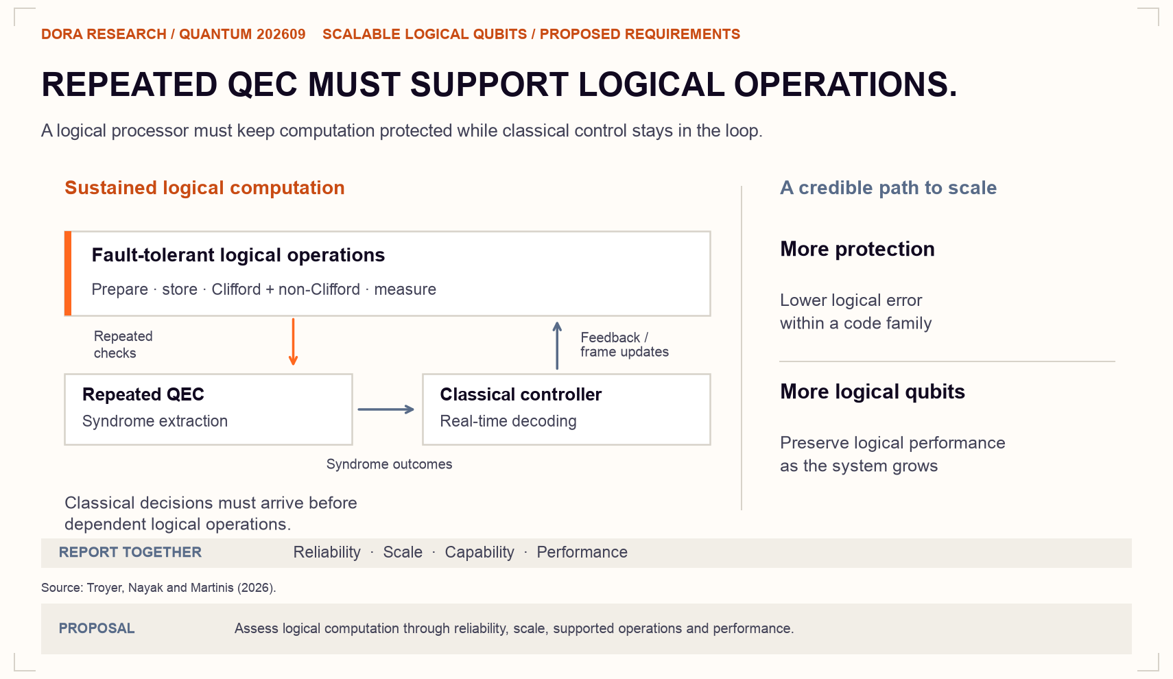
Troyer, Nayak and Martinis's proposed requirements connect logical operations, syndrome extraction, decoding and feedback with improving protection and scalable replication.[1]

Four dimensions of logical performance

The authors organize progress into four coupled dimensions.[1] Each adds information that a logical-qubit count leaves unspecified.

With a fixed physical-qubit budget, a team can encode more logical qubits at modest protection or fewer at stronger protection. A larger logical count can therefore accompany a higher error rate. The useful choice depends on the circuit: a wide, shallow workload and a narrow, deep workload may prefer different allocations.

Time introduces another trade-off. A decoder can improve its decisions by using more computation, but the controller still needs those decisions before dependent quantum operations proceed. A code with low spatial overhead can also require more steps to implement a logical gate. Reporting the cycle time alongside the full logical-operation latency makes these costs visible.

For demanding workloads, the authors discuss logical error targets around –, depending on the application and its allowed failure probability.[1]

From memory to universal control

The capability checklist covers logical state preparation and measurement, memory, Clifford operations, non-Clifford operations and measurement-conditioned control.[1] Researchers need to establish which of these work under repeated correction and how their errors accumulate when combined.

Non-Clifford operations often require magic states. A processor prepares an ancillary resource state and consumes it to implement a gate outside the Clifford set. State preparation can fail or require repeated attempts, and injection may need a correction conditioned on a measurement. A useful benchmark should include the cost of this sequence along with the quality of the final gate.

Postselection and error mitigation can improve particular tasks. Discarding runs with detected errors raises the quality of the retained data, while mitigation uses additional samples and a noise model to recover information from imperfect circuits. Their contribution to performance depends on how many executions the user needs. A logical result with excellent conditional fidelity should therefore also report its retention probability and time cost.

Once a processor supports the required instructions, a user needs to know which circuit shapes it can execute at acceptable quality and how much time those executions take. QUOPS supplies a common test for a specified family of circuits.

3. QUOPS: circuit size and effective throughput

A common circuit family

Gate fidelity measures local operations. Quantum Volume tests whole circuits by finding the largest passing square circuit, with equal width and depth. QUOPS allows width and size to vary independently and adds a measure of effective throughput.[2] Researchers can use it to compare the behavior of different execution stacks, including compilation, routing and logical encoding.

QUOPS stands for quantum universal operation performance system. Its circuits alternate random single-qubit Pauli rotations with CNOT layers on randomly paired qubits. The rotation axis and angle vary, and the CNOT pairs can span the circuit. Each platform compiles this shared instruction set into its own operations.

That compilation carries physical consequences. A device with local connectivity must route a CNOT between distant qubits. A Clifford+ processor must approximate an arbitrary-angle rotation using a sequence of discrete gates. Both routing errors and synthesis error reduce the quality of the implemented circuit. The benchmark includes those costs in the result.

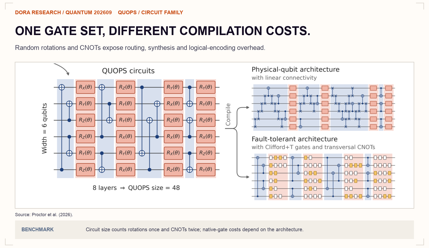
A common circuit family incurs different compilation costs on physical-qubit and fault-tolerant architectures. Proctor et al.[2]

The authors choose rotation-heavy circuits partly because they resemble product-formula Hamiltonian simulation. For algorithms dominated by Toffoli gates, we use the paper's non-Clifford resource conversion below.

Width, size and circuit quality

Circuit width counts the qubits on which the benchmark acts. Circuit size counts the operations in the shared gate set:

One single-qubit rotation contributes one unit; a CNOT contributes two. For a dense circuit of complete layers, is approximately width times depth. Compiling that circuit can require many more native operations. The logical implementation may also consume physical qubits for correction and ancillary states beyond the qubits carrying the benchmark computation.

At each , the researchers sample random circuits and estimate their mean process polarization . This quantity expresses the quality of the implemented quantum process relative to the intended one. The standard threshold is

All circuit shapes that pass this process-quality threshold form a capability region. A device can support wide circuits of limited size and much larger circuits at narrower widths.

Mirror circuits make quality measurable

A generic large random circuit can be expensive to simulate on a classical computer, which makes direct verification difficult. Proctor et al. use mirror circuit fidelity estimation, or MCFE.[2] The experiment embeds a circuit in a randomized mirror construction with a known ideal output. Reference circuits allow the analysis to estimate the quality of the original circuit while accounting for the additional operations used in the measurement procedure.

The mirror return probability contains errors from the whole constructed sequence. MCFE uses reference measurements and its compilation rules to estimate the original circuit's quality, avoiding a classical calculation of its full output distribution. The score tests use a confidence level of at least 95%.

From a region to one score

The headline QUOPS score is the largest passing size within

This restriction selects an admissible range of circuit shapes. It prevents extremely narrow or shallow circuits from dominating the headline score and reflects the shapes of the challenge problems chosen by the authors. The full region remains useful because two machines can obtain similar maximum scores at different widths.

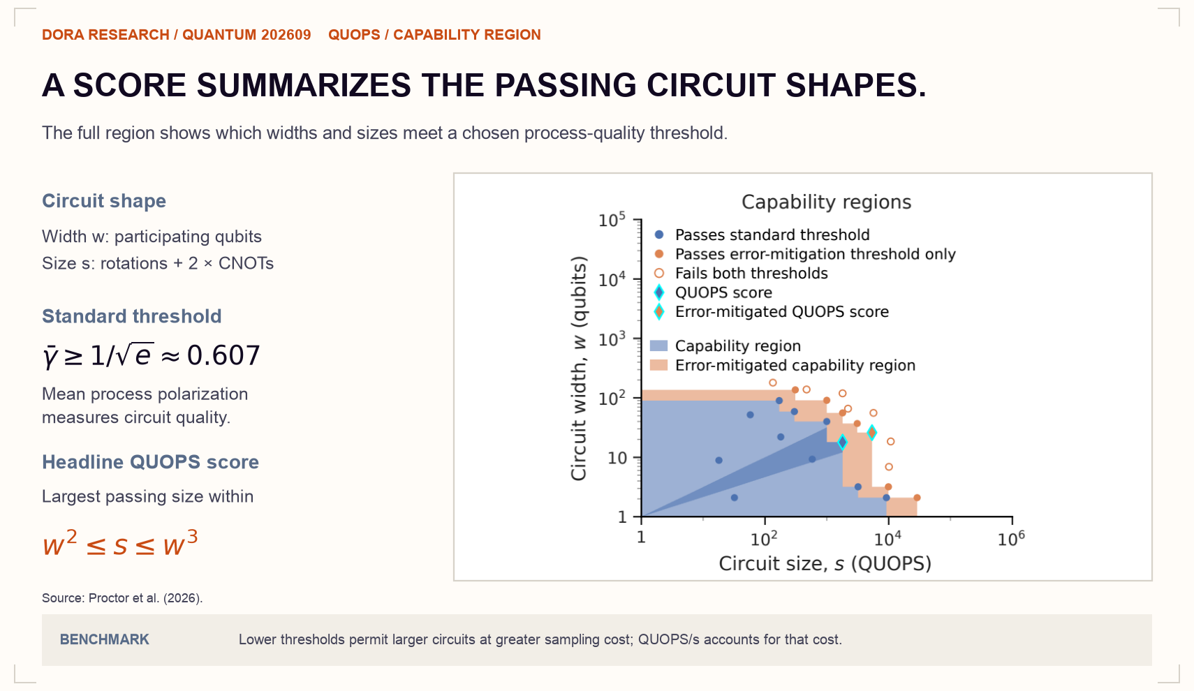
Standard and lower-threshold capability regions. Lowering the quality threshold permits larger circuits at additional sampling cost. Proctor et al.[2]

The notation also differs from the Quops used in the neutral-atom strategic plan discussed in our August newsletter.[9] That work counts operations on a logical-cycle basis. Here QUOPS size uses the rotation/CNOT definition above. Resource comparisons require an explicit conversion between the two conventions.

Effective throughput includes the sampling cost

A circuit score leaves execution time unspecified. Proctor et al. therefore report a QUOPS rate, expressed in QUOPS per second. Its idealized form is

where is the time per retained sample. The polarization factor accounts for the approximate sampling overhead needed to extract information from noisy results. The experimental definition also handles mirror length, postselection and batch timing.[2]

The authors illustrate the trade-off by lowering the threshold to . At this quality, the approximate sampling overhead is . A processor may then support a larger circuit, but the user pays for it through repeated execution. On Helios-1, the reported lower-threshold score reaches 20,442 QUOPS at 0.29 QUOPS/s, using a combination of direct measurements and extrapolation. The standard physical-qubit result is 1,504 QUOPS at 303 QUOPS/s. These two operating points describe different sampling budgets.

Hardware results separate scale from speed

The experiments cover Google Willow, IBM Boston and Quantinuum's H2-1 and Helios-1. Table 1 reproduces the paper's standard-threshold results.[2] Each rate corresponds to the circuit shape that gives the score in the same row.

Table 1. Measured QUOPS scores and effective rates.

Willow and Boston reach similar maximum sizes, while Willow has much higher effective throughput at its reported operating point. The trapped-ion systems sustain larger circuits but execute them at lower rates. Their all-to-all connectivity reduces the routing burden of random CNOT pairs. In the locally connected superconducting devices, routing becomes more expensive as the circuit widens.

The rates include experimental choices as well as hardware timing. Willow's throughput experiment uses large batches of repeated shots to amortize circuit-switching costs. IBM's rate uses a batch-time approximation, and the Quantinuum timing includes operational overheads within the measurement window.[2]

Widths of 6 or 16 identify the shapes that maximize the score. The processors can run wider circuits at other sizes. Their full capability regions contain this information, which the single-number summary omits.

The measured cost of fault tolerance

On Helios-1, the researchers also execute the benchmark on up to eight Steane logical qubits.[2] They implement Clifford gates transversally and supply gates through magic-state injection. The final version protects the circuit against a fault at any single location, including errors that can propagate between composed gate operations.

This implementation reaches 40 QUOPS at width 4 and 4.9 QUOPS/s. The score includes the errors and time costs of logical control and rotation synthesis. The original size-40 circuits contain 20 arbitrary-angle rotations, which the chosen synthesis approximates using an average of 10 gates before mirroring.

Successive implementations show how the benchmark can track software improvements on fixed hardware. Better magic states and synthesis randomization raise the score from 24 to 40. Revised QEC placement and improved parallel execution then increase the rate from 1.3 to 4.9 QUOPS/s while strengthening composable fault tolerance.[2]

The encoded implementation has a lower score than the physical-qubit implementation. Its small code and synthesis overhead define the measured operating point. To examine how larger protected systems could improve on it, the authors project the capability regions of two fault-tolerant architecture families.

4. Fault-tolerant capability and application resources

Two architecture models

Proctor et al. plot projected hardware capability against circuit size on the horizontal axis and width on the vertical axis, both on logarithmic scales.[2] Each shaded region represents predicted passing circuits at a specified physical-qubit budget . For the encoded regions, is the logical circuit width. The budget must also support syndrome extraction and ancillary resources.

The degree-4 architecture uses rotated surface codes, lattice-surgery CNOTs and cultivated states. The authors estimate costs with a simplified FLASQ model and set both one- and two-qubit gate error rates to . Increasing the physical budget from 5,000 to 50,000 qubits raises the predicted headline score from about to .

The common cutoff near size comes from the quality of the cultivated states. Their residual errors limit the circuit size even as the model adds protection to data qubits. The authors note that distillation could permit larger circuits, at additional resource cost.[2]

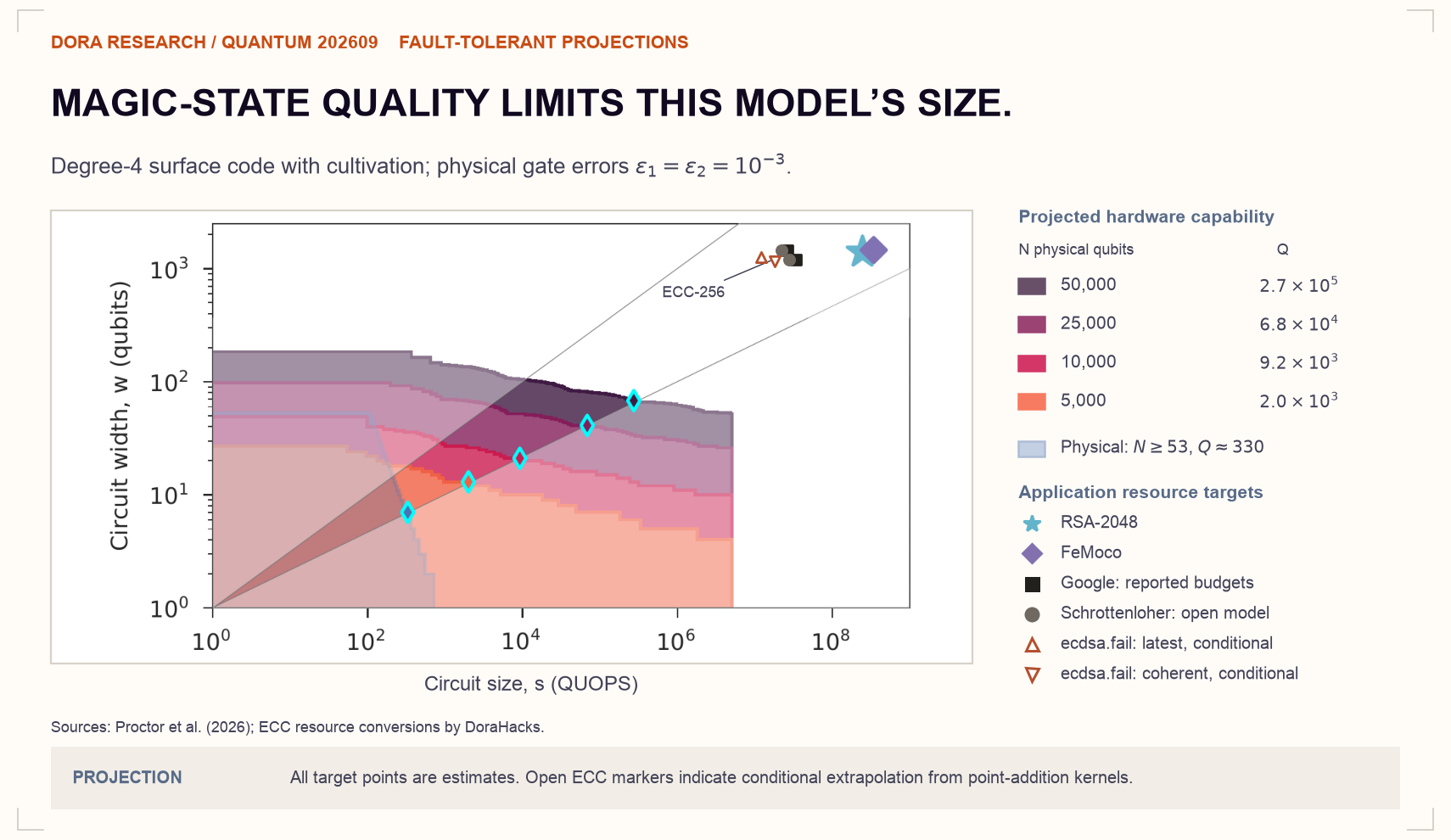
The fully connected architecture assumes one-qubit gate errors of and two-qubit gate errors of . It selects the best performance among a small set of surface-code and concatenated symplectic double-code constructions. With 10,000 physical qubits, the predicted score reaches about .[2] Compared with the degree-4 model, this architecture combines full connectivity with lower gate errors.

The blue regions show the corresponding unencoded models, whose scores saturate near 330 and , respectively. Error correction permits much larger circuits. The full-connectivity model reaches its maximum score at about a hundred logical qubits, while the application targets below require roughly a thousand or more.

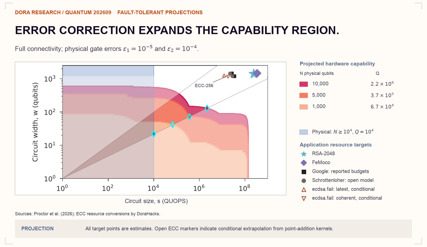
Converting application resources to QUOPS

The original figure places two application targets beside these regions: RSA-2048 factoring and energy estimation for a 76-orbital FeMoco model.[2–4] Both algorithms consume large numbers of Toffoli gates. QUOPS instead counts rotations and CNOTs, so the authors compare their non-Clifford resource requirements.

They first use a resource cost of four gates per Toffoli, appropriate to the compute/uncompute constructions assumed in the estimate. They then determine the -gate quality needed for the algorithm to meet the chosen polarization threshold and optimize the balance between rotation-synthesis error and -gate execution error. The model neglects Clifford and idle errors.

We reproduce this conversion for RSA and FeMoco, then apply it to secp256k1. Table 2 keeps the original logical resources beside the converted size. Width includes the algorithm's data and working registers. An architecture model then translates these logical resources into physical qubits, including factories, routing and QEC overhead.

Table 2. Application resources mapped to the QUOPS circuit basis. Toffoli counts refer to one algorithm circuit under the cited model. The ECC QUOPS values are our conversions using Proctor et al.'s method.

Gidney's factoring estimate includes an average of 9.2 circuit executions and about Toffolis in total.[3] We divide that total by 9.2 before mapping the single-circuit size. Proctor's five-day runtime comparison accounts for repetition when deriving a target rate of about QUOPS/s for RSA and for FeMoco.[2] Those target rates use raw size divided by time, whereas the device rate includes the polarization-squared adjustment.

Google and Schrottenloher provide two ECC working points each

Babbush et al., with authors from Google Quantum AI, the Ethereum Foundation and Stanford, report secp256k1 constructions below 1,200 logical qubits and 90 million Toffolis, or below 1,450 qubits and 70 million Toffolis.[5] They disclose resource budgets and a zero-knowledge verification procedure while keeping the point-addition circuits private. We plot the rounded budget endpoints from the corrected v2 of the paper.

Schrottenloher publishes an open point-addition construction and a complete-algorithm resource model.[6] Adding the 16-bit window register gives widths of 1,208 and 1,462 for the low-width and low-Toffoli variants. Their converted sizes are about 27.3 million and 21.9 million QUOPS.

For both sources, the low-width construction uses more Toffolis, while the low-Toffoli construction uses more qubits.

Mapping the latest ECDSA.Fail kernels to QUOPS

The public ECDSA.Fail challenge optimizes a reversible secp256k1 point-addition kernel and ranks submissions by peak live qubits multiplied by average executed Toffolis.[7,8] At our check on 28 September 2026, 13:06 Hong Kong time, the best product record uses 1,250 qubits and 889,047 Toffolis per point addition. The corresponding code commit is 03d9ecd.[8]

For the full-algorithm estimate, we assume a coherent 16-bit window adapter for this kernel and a schedule of 28 point-addition calls, with a lookup cost of 196,608 Toffolis per call:

The same non-Clifford conversion gives QUOPS, shown as an open triangle in the resource comparison.

ECDSA.Fail also reports an implemented coherent-window kernel for an earlier construction, using 1,162 qubits and about 1,684,161 Toffolis per call.[7] That kernel already includes the window register and lookup work. Applying the same 28-call schedule gives the separate -QUOPS target in Table 2.

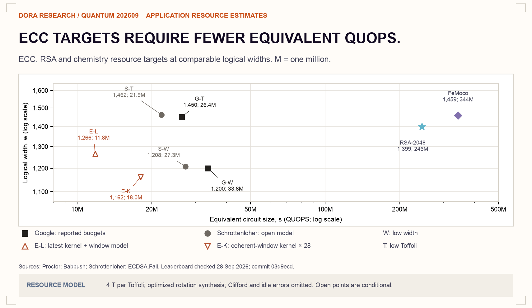
Application resource targets at comparable logical widths. Black squares denote Google budgets, gray circles denote Schrottenloher's resource models, and open orange triangles denote our conditional ECDSA.Fail extrapolations. W denotes the low-width variant and T the low-Toffoli variant. L (upward triangle) denotes the latest leaderboard kernel; K (downward triangle) denotes the implemented coherent-window kernel. The same six ECC targets appear on both architecture projections above, where the cyan diamonds mark the headline-score locations.[2,5–8]

Lower arithmetic cost still requires sufficient width

The ECC points lie to the left of the original RSA and FeMoco targets. Under the shared mapping, these selected secp256k1 constructions need a smaller equivalent circuit size. Their logical widths remain around 1,200–1,500. None lies within the projected capability regions shown here.

A processor must support the required size and width together. For the latest ECC target, that means a capability region covering QUOPS at a width of 1,266 logical qubits.

Hardware and QEC improvements can expand the shaded regions; better arithmetic can lower an application's resource demand. Google's budgets, Schrottenloher's open constructions and the ECDSA.Fail records show how algorithm development changes the target. With the QUOPS mapping, we can compare those changes with improvements in hardware capability.

5. Conclusion

Troyer, Nayak and Martinis propose reporting logical qubits together with their reliability, supported operations, scaling behavior and performance.[1] Proctor et al. make part of this comparison measurable through a shared circuit family.[2] Their experiments show why circuit size and throughput need separate reporting, and why a small logical implementation can incur substantial overhead even when its operations satisfy fault-tolerance requirements.

The next benchmark milestone is a fault-tolerant implementation that exceeds the best physical implementation under the same standard. Current resource models place secp256k1 at roughly a thousand logical qubits and tens of millions of equivalent QUOPS. Recent point-addition optimizations lower the estimated size further. Measuring capability across the required widths will show how closely logical processors approach these application targets.

6. References

1. Troyer, M., Nayak, C. and Martinis, J. "Scalable logical qubits." arXiv:2609.20549v1 (2026). Paper.
2. Proctor, T. et al. "Benchmarking the computational power of quantum computers." arXiv:2609.12146v1 (2026). Paper. Application mapping: Supplementary Information V; architecture projections: Supplementary Information VI.
3. Gidney, C. "How to factor 2048 bit RSA integers with less than a million noisy qubits." arXiv:2505.15917v1 (2025). Paper.
4. Low, G. H. et al. "Fast quantum simulation of electronic structure by spectrum amplification." Physical Review X 15, 041016 (2025). Published paper. Resource inputs follow arXiv:2502.15882v1, Table 1, 76-orbital model, as used by Proctor et al.
5. Babbush, R. et al. "Securing Elliptic Curve Cryptocurrencies against Quantum Vulnerabilities: Resource Estimates and Mitigations." arXiv:2603.28846v2 (2026). Paper.
6. Schrottenloher, A. "Optimized Point Addition Circuits for Elliptic Curve Discrete Logarithms." arXiv:2606.02235v1 (2026). Paper.
7. Long, J. et al. "ECDSA.Fail: Open Autoresearch for Optimizing Elliptic-Curve Point Addition in Shor's Algorithm." arXiv:2609.09582v2 (2026). Paper. Coherent-window implementation: Section 5.2.3 and Supplemental Note F.
8. ECDSA.Fail, public point-addition challenge. Website, official benchmark API, code at commit 03d9ecd. Snapshot checked on 28 September 2026 at 13:06 HKT.
9. Menssen, A. J. et al. "Strategic Plan for Neutral Atom Quantum Computation." arXiv:2607.21554 (2026). Paper.